Spatial predictors

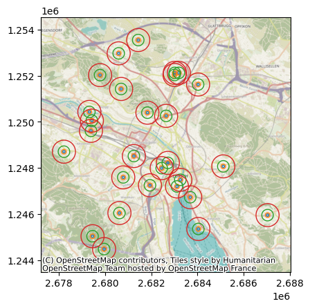
In the focal site multi-scale study framework (Brennen et al., 2002), a response variable (e.g., species abundance) is measured at multiple sites and the predictor variables are usually measures of landscape structure (e.g. habitat amount and configuration) computed at multiple spatial extents surrounding each focal site. The utility of such a framework transcends species-landscape relationships - in fact, land use regressions to predict air quality or temperature based on multi-scale spatial predictors fundamentally share the same setup (Hoek et al., 2008).

A key aspect of focal site multi-scale studies is the selection of spatial predictors, which are ultimately used as explanatory variables to study the effect of spatial pattern on a response variable.

Formal definition

Let \(\mathcal{S} = \{s_1, \ldots, s_n\}\) be a set of \(n\) sampling sites, each located at geographic coordinates \(\mathbf{p}_i \in \mathbb{R}^2\), and let \(y_i \in \mathbb{R}\) be an environmental response variable (e.g. air temperature, species richness) measured at site \(s_i\).

For site \(s_i\), a spatial predictor \(k\) at spatial extent (buffer radius) \(r\) is a vector summary of the environmental layer \(\mathcal{L}\) (raster or vector dataset) within the neighbourhood \(B(\mathbf{p}_i, r)\):

\[\mathbf{x}_{ikr} = f_k\bigl(\mathcal{L}\big|_{B(\mathbf{p}_i,\, r)}\bigr) \in \mathbb{R}^{d_k}\]

where \(f_k\) is an aggregation function (e.g. mean, sum, a landscape metric, or a learned embedding) and \(d_k \geq 1\) is the output dimension (\(d_k = 1\) for scalar summaries, \(d_k > 1\) for vector embeddings). Concatenating all \(K\) predictors across \(R\) spatial extents yields the feature matrix

\[\mathbf{X} \in \mathbb{R}^{n \times D}, \quad D = \sum_{k=1}^{K} d_k \cdot R\]

which is subsequently used to fit a model \(\hat{y} = g(\mathbf{X})\) relating landscape structure to the response variable.

import contextily as cx
import geopandas as gpd
import matplotlib.pyplot as plt
import rasterio as rio
import seaborn as sns

import focalpy

stations_filepath = "data/stations.gpkg"

buildings_filepath = "data/buildings.gpkg"
tree_canopy_filepath = "data/tree-canopy.tif"
dem_filepath = "data/dem.tif"
lulc_filepath = "data/lulc.tif"
tessera_filepath = "data/tesserach-zurich.tif"

buffer_dists = [50, 100, 250, 500]

stations_gdf = gpd.read_file(stations_filepath).set_index("station_id")

fig, ax = plt.subplots()
for buffer_dist, color in zip(buffer_dists, sns.color_palette()):
    stations_gdf.buffer(buffer_dist).plot(
        facecolor=(0, 0, 0, 0), edgecolor=color, ax=ax
    )
cx.add_basemap(ax, crs=stations_gdf.crs)

# buildings
buildings_gdf = gpd.read_file(buildings_filepath).set_index("id")
# add a "volume" column
buildings_gdf["volume"] = buildings_gdf["area"] * buildings_gdf["height"]
buildings_gdf.head()

	height	area	geometry	volume
id
4264	18.670619	10340.626863	POLYGON ((2680693.885 1251498.715, 2680695.967...	193065.902368
4436	16.988255	5692.331205	POLYGON ((2682125.575 1247611.584, 2682110.688...	96702.775194
4633	21.344529	3200.633956	POLYGON ((2683816.74 1248231.125, 2683816.581 ...	68316.025064
7565	23.081217	3083.217221	POLYGON ((2683434.771 1248110.727, 2683434.099...	71164.405863
57243	15.070181	1032.077993	POLYGON ((2683508.7 1247190.211, 2683519.131 1...	15553.602132

# dem
with rio.open(dem_filepath) as src:
    # read the one and only band
    dem_arr = src.read(1)
    dem_transform = src.transform
    dem_nodata = src.nodata

Computing features

fa = focalpy.FocalAnalysis(
    [buildings_gdf, tree_canopy_filepath, dem_filepath],
    stations_gdf,
    buffer_dists,
    [
        "compute_vector_features",
        "compute_raster_features",
        "compute_terrain_attributes",
    ],
    feature_col_prefixes=["building", "tree", ""],
    feature_methods_args={
        "compute_vector_features": [{"volume": "sum"}],
        "compute_terrain_attributes": [["slope", "topographic_position_index"]],
    },
    feature_methods_kwargs={
        "compute_raster_features": {"stats": "sum"},
        "compute_terrain_attributes": {"stats": "mean"},
    },
)
fa.features_df.head()

	building_volume_sum_50	building_volume_sum_100	building_volume_sum_250	building_volume_sum_500	tree_sum_50	tree_sum_100	tree_sum_250	tree_sum_500	slope_mean_50	slope_mean_100	slope_mean_250	slope_mean_500	topographic_position_index_mean_50	topographic_position_index_mean_100	topographic_position_index_mean_250	topographic_position_index_mean_500
station_id
2651	42799.252900	130087.412717	5.394371e+05	1.874661e+06	650.0	2281.0	12913.0	59364.0	6.258385	5.147757	3.865617	3.948312	0.002324	0.001576	0.000070	-0.000084
2652	28891.012664	100381.131949	6.930643e+05	2.925047e+06	134.0	1607.0	10679.0	38572.0	3.295830	3.792125	3.354241	3.435203	-0.000874	0.000531	-0.000046	-0.000022
2653	8218.052929	39102.191933	3.850106e+05	1.081819e+06	845.0	3211.0	18900.0	83168.0	6.053758	5.753644	6.210232	8.461916	0.000385	0.000706	0.000689	0.000174
2655	69366.625859	330706.307361	1.378667e+06	4.091401e+06	149.0	1005.0	9609.0	33100.0	1.742169	1.645347	2.092990	3.686358	-0.000051	-0.000204	-0.000106	-0.000154
2656	0.000000	360.659244	8.534503e+03	1.080769e+04	1950.0	7070.0	40955.0	172565.0	27.618801	29.190599	28.890853	29.256348	0.011389	0.003584	0.002101	0.000425

Vector data

Basic aggregation with GeoPandas

Vector datasets such as building footprints or road networks provide essential descriptors of the built environment and land use. Spatial predictors can be obtained by spatially joining each focal buffer with the vector layer and computing summary statistics (e.g., count, sum, mean…) of the polygon attributes within each buffer, for instance the total built-up area or the mean building height. To that end, we can use the focalpy.compute_vector_features functions, which wraps standard GeoPandas groupby/aggregate operations. For instance, we can compute the number of buildings by getting the "size" of each group:

focalpy.compute_vector_features(
    buildings_gdf, stations_gdf, buffer_dists, gb_reduce_method="size"
)

		size
station_id	buffer_dist
2651	50	6.0
	100	19.0
	250	124.0
	500	552.0
2652	50	8.0
...	...	...
SMA	500	555.0
UEB	50	2.0
	100	2.0
	250	20.0
	500	32.0

112 rows × 1 columns

We can also compute the per-buffer mean of each column:

focalpy.compute_vector_features(buildings_gdf, stations_gdf, buffer_dists, "mean")

		height_mean	area_mean	volume_mean
station_id	buffer_dist
2651	50	16.863535	423.278173	7133.208817
	100	15.645063	427.571637	6846.705932
	250	10.056238	339.999499	4350.298985
	500	8.837930	278.871534	3396.125261
2652	50	18.997770	191.284786	3611.376583
...	...	...	...	...
SMA	500	8.645853	192.181419	1837.771486
UEB	50	2.683603	183.051163	973.190031
	100	2.683603	183.051163	973.190031
	250	9.355363	167.553049	1246.004972
	500	9.658524	132.610983	984.392390

112 rows × 3 columns

aggregate each column differently:

focalpy.compute_vector_features(
    buildings_gdf, stations_gdf, buffer_dists, {"area": "sum", "height": "mean"}
)

		area_sum	height_mean
station_id	buffer_dist
2651	50	2539.669037	16.863535
	100	8123.861097	15.645063
	250	42159.937823	10.056238
	500	153937.086847	8.837930
2652	50	1530.278291	18.997770
...	...	...	...
SMA	500	106660.687706	8.645853
UEB	50	366.102327	2.683603
	100	366.102327	2.683603
	250	3351.060986	9.355363
	500	4243.551471	9.658524

112 rows × 2 columns

or compute several aggregations for all columns:

focalpy.compute_vector_features(
    buildings_gdf, stations_gdf, buffer_dists, ["sum", "mean"]
)

		height_sum	height_mean	area_sum	area_mean	volume_sum	volume_mean
station_id	buffer_dist
2651	50	101.181213	16.863535	2539.669037	423.278173	4.279925e+04	7133.208817
	100	297.256202	15.645063	8123.861097	427.571637	1.300874e+05	6846.705932
	250	1246.973527	10.056238	42159.937823	339.999499	5.394371e+05	4350.298985
	500	4878.537480	8.837930	153937.086847	278.871534	1.874661e+06	3396.125261
2652	50	151.982158	18.997770	1530.278291	191.284786	2.889101e+04	3611.376583
...	...	...	...	...	...	...	...
SMA	500	4798.448197	8.645853	106660.687706	192.181419	1.019963e+06	1837.771486
UEB	50	5.367206	2.683603	366.102327	183.051163	1.946380e+03	973.190031
	100	5.367206	2.683603	366.102327	183.051163	1.946380e+03	973.190031
	250	187.107254	9.355363	3351.060986	167.553049	2.492010e+04	1246.004972
	500	309.072774	9.658524	4243.551471	132.610983	3.150056e+04	984.392390

112 rows × 6 columns

we can further estimate the building volume as a product of the area and height and compute its mean:

focalpy.compute_vector_features(
    buildings_gdf.assign(**{"volume": buildings_gdf["area"] * buildings_gdf["height"]}),
    stations_gdf,
    buffer_dists,
    {"volume": "mean"},
)

		volume_mean
station_id	buffer_dist
2651	50	7133.208817
	100	6846.705932
	250	4350.298985
	500	3396.125261
2652	50	3611.376583
...	...	...
SMA	500	1837.771486
UEB	50	973.190031
	100	973.190031
	250	1246.004972
	500	984.392390

112 rows × 1 columns

Urban morphometrics with momepy

Beyond simple aggregations, momepy (Fleischmann, 2019) provides a comprehensive toolkit of urban morphometric indicators that characterise the shape, size, and spatial arrangement of urban elements. These include measures of compactness (e.g. circular compactness), elongation, fractal dimension and many others that capture the three-dimensional complexity of the built environment. focalpy wraps momepy metrics via compute_urban_morphometrics, computing and aggregating them within each focal buffer. We only need to provide the list of target momepy metrics and aggregation function:

focalpy.compute_urban_morphometrics(
    buildings_gdf,
    stations_gdf,
    buffer_dists,
    ["circular_compactness", "fractal_dimension"],
    "mean",
)

		circular_compactness_mean	fractal_dimension_mean
station_id	buffer_dist
2651	50	0.553636	1.022197
	100	0.550181	1.023150
	250	0.538925	1.030278
	500	0.519466	1.041202
2652	50	0.538450	1.022200
...	...	...	...
SMA	500	0.550440	1.034010
UEB	50	0.700509	0.916253
	100	0.700509	0.916253
	250	0.517528	1.049154
	500	0.530266	1.046731

112 rows × 2 columns

it is also possible to pass keyword arguments to each momepy function:

focalpy.compute_urban_morphometrics(
    buildings_gdf,
    stations_gdf,
    buffer_dists,
    ["circular_compactness", "form_factor"],
    "mean",
    momepy_metrics_kwargs_dict={"form_factor": {"height": buildings_gdf["height"]}},
)

		circular_compactness_mean	form_factor_mean
station_id	buffer_dist
2651	50	0.553636	5.146849
	100	0.550181	5.183737
	250	0.538925	36.460616
	500	0.519466	15.382184
2652	50	0.538450	5.587796
...	...	...	...
SMA	500	0.550440	5.911815
UEB	50	0.700509	19.259741
	100	0.700509	19.259741
	250	0.517528	24.733243
	500	0.530266	17.679633

112 rows × 2 columns

Raster data

Zonal statistics with rasterstats

Raster layers - such as digital elevation models (DEM), land use/land cover (LULC) maps, or remote-sensing-derived indices - can be summarised within each focal buffer through zonal statistics, i.e. computing aggregate functions (mean, sum, min, max…) over the pixel values that fall within the buffer. To that end, focalpy uses rasterstats under the hood for this purpose via the compute_raster_features function. For instance, we can compute the mean altitude within each buffer by providing a raster DEM:

focalpy.compute_raster_features(
    dem_arr,
    stations_gdf,
    buffer_dists,
    affine=dem_transform,
    stats="mean",
    nodata=dem_nodata,
)

		mean
station_id	buffer_dist
2651	50	455.053617
	100	454.768099
	250	453.078239
	500	453.072617
2652	50	406.412919
...	...	...
SMA	500	560.063654
UEB	50	853.093014
	100	844.082015
	250	803.673862
	500	748.301653

112 rows × 1 columns

We can also use it to compute the sum and mean of pixels of a given LULC class, e.g., urban green spaces:

with rio.open(lulc_filepath) as src:
    # read the one and only band
    lulc_arr = src.read(1)
    lulc_transform = src.transform

target_class = 5  # urban green spaces
focalpy.compute_raster_features(
    lulc_arr == target_class,
    stations_gdf,
    buffer_dists,
    affine=lulc_transform,
    stats=["sum", "mean"],
)

/home/martibosch/libraries/focalpy/.pixi/envs/user-guide/lib/python3.13/site-packages/rasterstats/io.py:335: NodataWarning: Setting nodata to -999; specify nodata explicitly
  warnings.warn(

		mean	sum
station_id	buffer_dist
2651	50	0.000000	0.0
	100	0.000000	0.0
	250	0.000000	0.0
	500	0.000801	1.0
2652	50	0.000000	0.0
...	...	...	...
SMA	500	0.004785	6.0
UEB	50	0.000000	0.0
	100	0.000000	0.0
	250	0.000000	0.0
	500	0.000000	0.0

112 rows × 2 columns

Landscape metrics with PyLandStats

Landscape ecology provides numerous metrics to quantify the spatial composition and configuration of habitat patches, including proportion of landscape, edge density, patch shape complexity, and diversity indices (Riitters, 2019). In focalpy, the compute_landscape_metrics function enables easy computation of landscape metrics for each buffer using PyLandStats (Bosch, 2019). For instance, we can provide a list of class-level and landscape-level metrics as well as a list of classes to include:

# green spaces (5), meadows/pastures (8) and forests (10)
focalpy.compute_landscape_metrics(
    lulc_filepath,
    stations_gdf,
    buffer_dists,
    class_metrics=["proportion_of_landscape", "edge_density"],
    landscape_metrics=["shannon_diversity_index"],
    classes=[5, 8, 10],
)

[########################################] | 100% Completed | 102.04 ms
[########################################] | 100% Completed | 100.99 ms
[                                        ] | 0% Completed | 150.59 us

/home/martibosch/libraries/focalpy/.pixi/envs/user-guide/lib/python3.13/site-packages/pylandstats/landscape.py:3533: RuntimeWarning: Entropy-based metrics can only be computed in landscapes with at least two classes of patches. Returning nan
  warnings.warn(
/home/martibosch/libraries/focalpy/.pixi/envs/user-guide/lib/python3.13/site-packages/pylandstats/landscape.py:3533: RuntimeWarning: Entropy-based metrics can only be computed in landscapes with at least two classes of patches. Returning nan
  warnings.warn(

[########################################] | 100% Completed | 101.35 ms
[########################################] | 100% Completed | 303.72 ms
[########################################] | 100% Completed | 206.85 ms
[########################################] | 100% Completed | 100.87 ms
[########################################] | 100% Completed | 212.66 ms
[########################################] | 100% Completed | 101.74 ms

		proportion_of_landscape_5	proportion_of_landscape_8	proportion_of_landscape_10	edge_density_5	edge_density_8	edge_density_10	shannon_diversity_index
station_id	buffer_dist
2651	50	0.000000	0.000000	0.000000	0.000000	0.000000	0.000000	0.691416
	100	0.000000	0.000000	0.000000	0.000000	0.000000	0.000000	0.655178
	250	0.000000	1.935484	0.000000	0.000000	16.774194	0.000000	0.833076
	500	0.080064	5.364291	0.000000	1.281025	31.385108	0.000000	0.933643
2652	50	0.000000	0.000000	0.000000	0.000000	0.000000	0.000000	0.529706
...	...	...	...	...	...	...	...	...
SMA	500	0.478469	0.956938	8.213716	2.551834	8.293461	24.880383	1.193421
UEB	50	0.000000	0.000000	76.923077	0.000000	0.000000	184.615385	0.676720
	100	0.000000	0.000000	78.431373	0.000000	0.000000	156.862745	0.735071
	250	0.000000	0.000000	66.773163	0.000000	0.000000	173.801917	1.054298
	500	0.000000	0.556881	75.417661	0.000000	3.500398	144.789181	0.827920

112 rows × 7 columns

Terrain attributes with xDEM

Topography exerts a strong influence on many environmental processes, from cold-air drainage in urban valleys to hydrological connectivity and solar radiation exposure. Terrain attributes such as slope, aspect, curvature, and the topographic position index (TPI) can be derived from a digital elevation model (DEM). To that end, focalpy uses xDEM (Hugonnet et al., 2022) to compute these attributes and then aggregates them within each focal buffer via the compute_terrain_attributes function. For example, we can compute the mean and max slope for each site and buffer:

focalpy.compute_terrain_attributes(
    dem_filepath, stations_gdf, buffer_dists, "slope", stats=["mean", "max"]
)

		slope_mean	slope_max
station_id	buffer_dist
2651	50	6.258385	46.536942
	100	5.147757	46.536942
	250	3.865617	50.672459
	500	3.948312	50.672459
2652	50	3.295830	26.684357
...	...	...	...
SMA	500	10.515907	61.013931
UEB	50	7.556008	47.828327
	100	20.953310	71.454239
	250	30.595184	79.063553
	500	29.370031	79.063553

112 rows × 2 columns

or compute several metrics, e.g., adding TPI:

focalpy.compute_terrain_attributes(
    dem_filepath,
    stations_gdf,
    buffer_dists,
    ["slope", "topographic_position_index"],
    stats="mean",
)

		slope_mean	topographic_position_index_mean
station_id	buffer_dist
2651	50	6.258385	0.002324
	100	5.147757	0.001576
	250	3.865617	0.000070
	500	3.948312	-0.000084
2652	50	3.295830	-0.000874
...	...	...	...
SMA	500	10.515907	-0.000143
UEB	50	7.556008	0.015926
	100	20.953310	0.015927
	250	30.595184	0.004503
	500	29.370031	0.001672

112 rows × 2 columns

Additionally, we can aggregate each attribute differently by providing a list of stats that positionally match the list of metrics:

focalpy.compute_terrain_attributes(
    dem_filepath,
    stations_gdf,
    buffer_dists,
    ["slope", "topographic_position_index"],
    stats=["mean", "max"],
)

		slope_mean	slope_max	topographic_position_index_mean	topographic_position_index_max
station_id	buffer_dist
2651	50	6.258385	46.536942	0.002324	1.613647
	100	5.147757	46.536942	0.001576	1.613647
	250	3.865617	50.672459	0.000070	1.746887
	500	3.948312	50.672459	-0.000084	1.901245
2652	50	3.295830	26.684357	-0.000874	0.532562
...	...	...	...	...	...
SMA	500	10.515907	61.013931	-0.000143	3.343628
UEB	50	7.556008	47.828327	0.015926	0.703735
	100	20.953310	71.454239	0.015927	2.174011
	250	30.595184	79.063553	0.004503	6.606323
	500	29.370031	79.063553	0.001672	6.606323

112 rows × 4 columns

Embedding features

Foundation models for Earth observation learn compact, semantically rich representations of the landscape directly from satellite time series, without requiring hand-crafted feature engineering. In focalpy, geoembeddings from foundational models can be used as multi-scale focal predictors via compute_raster_features with the indexes parameter, which treats each embedding dimension as a separate band and aggregates it within each focal buffer. For instance, we use the embeddings of the TESSERA (Feng et al., 2026) model (provided by the TesseraCH instance within the Swiss Data Cube (Giuliani et al., 2017)), which produces per-pixel 16-dimensional embeddings from Sentinel-2 imagery at 10 m resolution in EPSG:2056:

focalpy.compute_raster_features(
    tessera_filepath,
    stations_gdf,
    buffer_dists,
    indexes=range(1, 9),
    band_prefix="tessera",
    stats="mean",
)

/home/martibosch/libraries/focalpy/.pixi/envs/user-guide/lib/python3.13/site-packages/rasterstats/io.py:335: NodataWarning: Setting nodata to -999; specify nodata explicitly
  warnings.warn(

		tessera_1_mean	tessera_2_mean	tessera_3_mean	tessera_4_mean	tessera_5_mean	tessera_6_mean	tessera_7_mean	tessera_8_mean
station_id	buffer_dist
2651	50	7.892569	0.186058	-17.637870	-2.607904	0.613337	0.418400	-8.208691	8.698803
	100	7.801788	-0.283322	-17.009456	-3.153286	0.222913	0.181502	-8.099371	8.385496
	250	9.202094	-0.964912	-17.276590	-2.902726	-1.045133	1.306718	-6.896602	8.253628
	500	9.624077	-0.458643	-17.975421	-3.103112	-0.890727	1.544997	-6.428439	7.644577
2652	50	11.826660	-5.227532	-15.805838	-5.929575	-4.202278	-2.248786	-3.524276	12.881348
...	...	...	...	...	...	...	...	...	...
SMA	500	9.711702	4.309838	-17.336694	-2.147834	-0.544849	1.898409	-9.053722	7.642174
UEB	50	4.058430	7.008330	-16.849395	1.257009	-2.671455	4.563640	-4.611345	6.129853
	100	3.942891	6.943526	-15.037635	2.932227	-3.973046	5.616287	-6.288865	4.988400
	250	3.411806	3.192039	-15.017236	4.429847	-3.270214	5.941413	-7.680755	4.205943
	500	4.212605	5.104426	-14.209330	4.165118	-2.976318	5.433813	-7.133730	4.218562

112 rows × 8 columns