Landscape-species inference#
The central focus of landscape ecology is exploring the relationship between the spatial pattern of landscapes and the ecological processes that occur on them (Hesselbarth et al., 2024).
This notebook shows how the FocalAnalysis class can be used to perform landscape-species inference following the focal site multi-scale study framework (Brennen et al., 2002). As an example use case, we will explore the relationship between bird species richness collected at multiple sites in Zurich - data from (Casanelles-Abella et al., 2021) - and the spatial patterns of the landscape surrounding each site.
Note that the approach of this analysis is essentially the same as the `MultiScaleAnalysis class draft of pylandstats <martibosch/pylandstats-notebooks>`__. It is likely that in the near future many of the functionalities of the ``MultiScaleAnalysis`` (and also ``SpatialSignatureAnalysis``) class disappear from the pylandstats code base and are instead implemented in focalpy (and thus imported in pylandstats).
We will first import the required libraries and define some utility functions for plotting.
[ ]:
import warnings

import contextily as cx
import geopandas as gpd
import matplotlib.pyplot as plt
import pandas as pd
import statsmodels.api as sm
from scipy import stats
from sklearn import ensemble, feature_selection, linear_model, preprocessing
from sklearn.model_selection import cross_val_score

import focalpy
[ ]:
# spatial predictors
buildings_filepath = "data/buildings.gpkg"
lulc_filepath = "data/lulc.tif"
tree_canopy_filepath = "data/tree-canopy.tif"

# green spaces (5), meadows/pastures (8) and forests (10)
lulc_classes = [5, 8, 10]
class_metrics = ["proportion_of_landscape"]
landscape_metrics = ["shannon_diversity_index"]

# response
species_richness_filepath = "data/bird-richness.gpkg"
y_col = "n.species"  # species richness

# scales
buffer_dists = [250, 500, 750, 1000]  # in meters

# target area (for region-wide prediction/extrapolation)
study_area_filepath = "data/study-area.gpkg"
grid_res = 500

# viz
figwidth = plt.rcParams["figure.figsize"][0]
figheight = plt.rcParams["figure.figsize"][1]
Let us start by plotting the target variable, i.e., the number of bird species recorded at each site:
[ ]:
bird_gdf = gpd.read_file(species_richness_filepath)
# bird_gdf.head()

ax = bird_gdf.plot(y_col, legend=True, legend_kwds={"label": "N. species"})
cx.add_basemap(ax, crs=bird_gdf.crs)
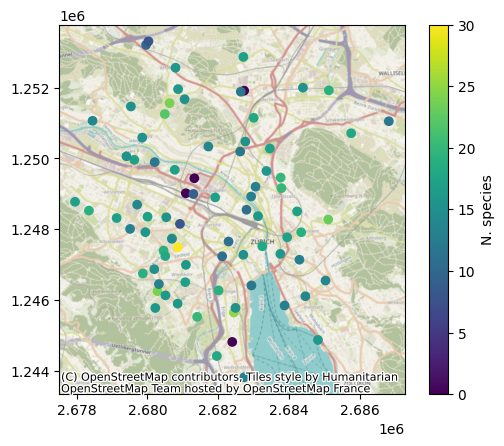
Since the analysis is performed in an urban landsape - which tend to have greater spatial heterogeneity (Band et al., 2005), we are using a version of the Swiss Land Statistics (SLS) datasets from the Swiss Federal Statistical Office whose resolution has been downscaled from the original 100 m to 25 m - see (Giuliani et al., 2022) for more details on the methods used. In order to simplify the analysis, we will use the aggregated 17-code LULC scheme from the NOAS04 nomenclature of the SLS datasets (link in French).
Following the variables defined above, we will instantiate a FocalAnalysis with the following multi-scale spatial predictors: the proportion of landscape covered the green spaces, meadows/pastures and forests as well as the Shannon diversity index (SHDI), which reflects the relative abundance of each LULC class:
[ ]:
fa = focalpy.FocalAnalysis(
    lulc_filepath,
    bird_gdf,
    buffer_dists,
    "compute_landscape_metrics",
    feature_methods_kwargs=dict(
        class_metrics=class_metrics,
        landscape_metrics=landscape_metrics,
        classes=lulc_classes,
    ),
)
[########################################] | 100% Completed | 315.31 ms
[########################################] | 100% Completed | 555.50 ms
[########################################] | 100% Completed | 314.31 ms
[########################################] | 100% Completed | 680.34 ms
[########################################] | 100% Completed | 425.79 ms
[########################################] | 100% Completed | 672.60 ms
[########################################] | 100% Completed | 419.86 ms
[########################################] | 100% Completed | 664.93 ms
The requested features will be stored as the features_df attribute:
[ ]:
fa.features_df.head()
| proportion_of_landscape_5_250 | proportion_of_landscape_5_500 | proportion_of_landscape_5_750 | proportion_of_landscape_5_1000 | proportion_of_landscape_8_250 | proportion_of_landscape_8_500 | proportion_of_landscape_8_750 | proportion_of_landscape_8_1000 | proportion_of_landscape_10_250 | proportion_of_landscape_10_500 | proportion_of_landscape_10_750 | proportion_of_landscape_10_1000 | shannon_diversity_index_250 | shannon_diversity_index_500 | shannon_diversity_index_750 | shannon_diversity_index_1000 | |
|---|---|---|---|---|---|---|---|---|---|---|---|---|---|---|---|---|
| zone | ||||||||||||||||
| 0 | 0.000000 | 1.037510 | 1.239377 | 3.189793 | 0.000000 | 0.000000 | 0.000000 | 0.737640 | 0.0 | 0.000000 | 0.000000 | 0.338915 | 0.715564 | 0.868716 | 0.896390 | 1.054748 |
| 1 | 0.000000 | 0.000000 | 2.547771 | 3.702966 | 0.634921 | 3.505976 | 3.326256 | 2.130201 | 0.0 | 7.649402 | 14.543524 | 18.893092 | 0.800883 | 1.140386 | 1.363838 | 1.422790 |
| 2 | 0.000000 | 0.000000 | 1.204392 | 6.135458 | 0.000000 | 0.000000 | 2.019129 | 1.852590 | 0.0 | 0.000000 | 1.487779 | 6.752988 | 0.625197 | 0.704713 | 0.952338 | 1.262781 |
| 3 | 18.910256 | 19.329073 | 15.313719 | 10.001992 | 0.000000 | 4.392971 | 4.253811 | 3.646145 | 0.0 | 1.038339 | 10.173697 | 16.796175 | 1.111966 | 1.326478 | 1.540855 | 1.573991 |
| 4 | 12.779553 | 23.248408 | 16.967765 | 11.080112 | 0.000000 | 0.477707 | 3.719447 | 4.184934 | 0.0 | 0.079618 | 2.833865 | 10.721403 | 0.959092 | 1.150802 | 1.423296 | 1.526619 |
We can get a first idea of the relationship between the spatial predictors and our target variable by inspecting the weights of a linear regression model estimated using the ordinary least squares (OLS) class of statsmodels:
[ ]:
X_df = fa.features_df
y_ser = bird_gdf[y_col]

results = sm.OLS(y_ser, sm.add_constant(X_df)).fit()
print(results.summary())
                            OLS Regression Results
==============================================================================
Dep. Variable:              n.species   R-squared:                       0.313
Model:                            OLS   Adj. R-squared:                  0.144
Method:                 Least Squares   F-statistic:                     1.848
Date:                Wed, 31 Dec 2025   Prob (F-statistic):             0.0430
Time:                        16:03:47   Log-Likelihood:                -234.91
No. Observations:                  82   AIC:                             503.8
Df Residuals:                      65   BIC:                             544.7
Df Model:                          16
Covariance Type:            nonrobust
===================================================================================================
                                      coef    std err          t      P>|t|      [0.025      0.975]
---------------------------------------------------------------------------------------------------
const                              21.2042      3.769      5.626      0.000      13.677      28.731
proportion_of_landscape_5_250      -0.0242      0.077     -0.313      0.755      -0.178       0.130
proportion_of_landscape_5_500       0.1827      0.283      0.645      0.521      -0.383       0.749
proportion_of_landscape_5_750      -0.0818      0.532     -0.154      0.878      -1.144       0.980
proportion_of_landscape_5_1000      0.4116      0.445      0.925      0.358      -0.477       1.300
proportion_of_landscape_8_250      -0.8318      0.529     -1.572      0.121      -1.888       0.225
proportion_of_landscape_8_500       0.3418      0.933      0.366      0.715      -1.521       2.205
proportion_of_landscape_8_750       0.1967      1.357      0.145      0.885      -2.514       2.908
proportion_of_landscape_8_1000     -0.1979      0.986     -0.201      0.842      -2.167       1.772
proportion_of_landscape_10_250      0.4349      0.387      1.124      0.265      -0.338       1.208
proportion_of_landscape_10_500     -0.7331      0.489     -1.501      0.138      -1.709       0.243
proportion_of_landscape_10_750      0.5792      0.573      1.011      0.316      -0.565       1.723
proportion_of_landscape_10_1000     0.2055      0.316      0.651      0.518      -0.425       0.836
shannon_diversity_index_250         9.6635      4.139      2.334      0.023       1.396      17.931
shannon_diversity_index_500        -6.7687      8.139     -0.832      0.409     -23.023       9.486
shannon_diversity_index_750        -0.7112     12.713     -0.056      0.956     -26.102      24.679
shannon_diversity_index_1000       -9.2402      9.040     -1.022      0.311     -27.294       8.814
==============================================================================
Omnibus:                       12.139   Durbin-Watson:                   1.367
Prob(Omnibus):                  0.002   Jarque-Bera (JB):               15.240
Skew:                          -0.691   Prob(JB):                     0.000490
Kurtosis:                       4.596   Cond. No.                         768.
==============================================================================

Notes:
[1] Standard Errors assume that the covariance matrix of the errors is correctly specified.
[ ]:
focalpy.scale_eval_ser(X_df, y_ser)
1000    0.182204
250     0.066968
500     0.092940
750     0.141639
Name: rsquared, dtype: float64
which suggests that the strongest effects occur when using focal buffers of a 1000 m radius. By default, the scale evaluation will be based on the coefficient of determination (R\(^2\)) of an ordinary least squares linear regression model. However, it is possible to use the model keyword argument to customize the criteria by providing any model from statsmodels or a function name of a statistical test from scipy.stats such as "spearmanr". Additionally, it is also possible
to determine the scale of effect for each feature separately by setting the how keyword argument to "individual" (see an example of this in the land use regression notebook).
In order to get the list of features at the scale of effect (based on the evaluation shown above), we can use the scale_of_effect_features, which will return the column names:
[ ]:
soe_features = focalpy.scale_of_effect_features(X_df, y_ser)
soe_features
Index(['proportion_of_landscape_5_1000', 'proportion_of_landscape_8_1000',
       'proportion_of_landscape_10_1000', 'shannon_diversity_index_1000'],
      dtype='object')
We can now use this to perform again our regression using only the features at the scale of effect:
[ ]:
X_soe_df = fa.features_df[soe_features]

results = sm.OLS(y_ser, sm.add_constant(X_soe_df)).fit()
print(results.summary())
                            OLS Regression Results
==============================================================================
Dep. Variable:              n.species   R-squared:                       0.182
Model:                            OLS   Adj. R-squared:                  0.140
Method:                 Least Squares   F-statistic:                     4.289
Date:                Wed, 31 Dec 2025   Prob (F-statistic):            0.00347
Time:                        16:03:52   Log-Likelihood:                -242.04
No. Observations:                  82   AIC:                             494.1
Df Residuals:                      77   BIC:                             506.1
Df Model:                           4
Covariance Type:            nonrobust
===================================================================================================
                                      coef    std err          t      P>|t|      [0.025      0.975]
---------------------------------------------------------------------------------------------------
const                              23.0950      3.396      6.801      0.000      16.333      29.857
proportion_of_landscape_5_1000      0.4260      0.147      2.898      0.005       0.133       0.719
proportion_of_landscape_8_1000      0.3574      0.355      1.006      0.318      -0.350       1.065
proportion_of_landscape_10_1000     0.2687      0.073      3.682      0.000       0.123       0.414
shannon_diversity_index_1000       -9.6640      3.212     -3.009      0.004     -16.060      -3.268
==============================================================================
Omnibus:                       18.910   Durbin-Watson:                   1.354
Prob(Omnibus):                  0.000   Jarque-Bera (JB):               34.948
Skew:                          -0.843   Prob(JB):                     2.58e-08
Kurtosis:                       5.718   Cond. No.                         115.
==============================================================================

Notes:
[1] Standard Errors assume that the covariance matrix of the errors is correctly specified.
We can see that this notably decreases our condition number (which is nonetheless still very high) but also at the expense of a decreased R\(^2\). At the same time, at this scale (1000 m) all the spatial predictors seem to have a significant effect except the proportion of meadows/pastures.
Note that besides the scale of effect, we can use any other method to select spatial predictors, e.g., methods designed for landscape metrics (Schindler et al., 2015) or filters, wrappers and embedded feature selection methods commonly used in machine learning models (Effrosynidis and Arampatzis, 2021). Given the pedagogical purposes of this example, we just show here how a sequential feature selector from scikit-learn can be used:
[ ]:
sfs_model = linear_model.LinearRegression()
sfs = feature_selection.SequentialFeatureSelector(sfs_model, n_features_to_select=4)
sfs_features = sfs.fit(X_df, y_ser).get_feature_names_out()
X_sfs_df = fa.features_df[sfs_features]

results = sm.OLS(y_ser, sm.add_constant(X_sfs_df)).fit()
print(results.summary())
                            OLS Regression Results
==============================================================================
Dep. Variable:              n.species   R-squared:                       0.057
Model:                            OLS   Adj. R-squared:                  0.008
Method:                 Least Squares   F-statistic:                     1.161
Date:                Wed, 31 Dec 2025   Prob (F-statistic):              0.335
Time:                        16:03:55   Log-Likelihood:                -247.89
No. Observations:                  82   AIC:                             505.8
Df Residuals:                      77   BIC:                             517.8
Df Model:                           4
Covariance Type:            nonrobust
==================================================================================================
                                     coef    std err          t      P>|t|      [0.025      0.975]
--------------------------------------------------------------------------------------------------
const                             14.0083      0.880     15.912      0.000      12.255      15.761
proportion_of_landscape_5_750      0.1887      0.109      1.726      0.088      -0.029       0.406
proportion_of_landscape_8_250     -0.1618      0.425     -0.381      0.704      -1.008       0.684
proportion_of_landscape_8_1000    -0.0113      0.340     -0.033      0.973      -0.688       0.666
proportion_of_landscape_10_250     0.2001      0.238      0.842      0.403      -0.273       0.674
==============================================================================
Omnibus:                       17.862   Durbin-Watson:                   1.138
Prob(Omnibus):                  0.000   Jarque-Bera (JB):               34.933
Skew:                          -0.764   Prob(JB):                     2.60e-08
Kurtosis:                       5.809   Cond. No.                         13.2
==============================================================================

Notes:
[1] Standard Errors assume that the covariance matrix of the errors is correctly specified.
While the sequential feature selection seems to successfully address the collinearity issue, the statistical strength is also vastly reduced.
Spatial extrapolation#
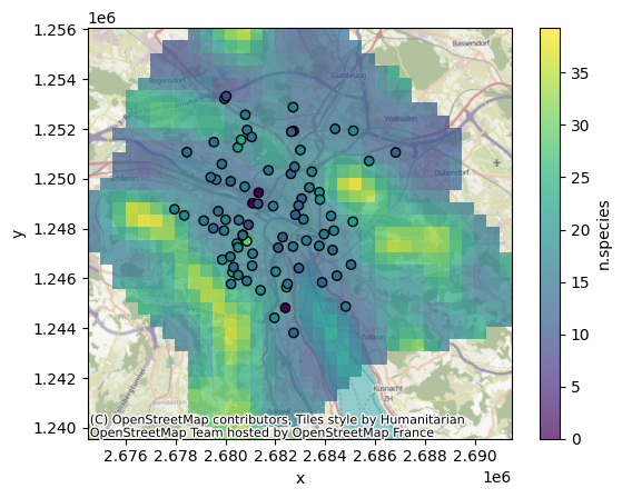
A key objective of the focal analysis design is to spatially extrapolate the inferred landscape-species relationships to a target study area. To that end, given a fitted scikit-learn model, we can use the predict_raster function by providing a vector data source defining the target area as well as the desired grid resolution:
[ ]:
model_class = linear_model.LinearRegression
model = model_class().fit(X_soe_df, y_ser)
# ax = scatterplot_obs_pred(
#     model,
#     X_soe_df,
#     y_ser,
# )
with warnings.catch_warnings():
    # ignore pylandstats warning when computing entropy-based metrics in landscapes with
    # only one LULC class
    warnings.simplefilter("ignore")
    pred_da = fa.predict_raster(
        model,
        study_area_filepath,
        grid_res,
        features=soe_features,
        pred_label=y_ser.name,
    )
focalpy.plot_raster_and_gdf(pred_da, bird_gdf, y_ser)
[########################################] | 100% Completed | 1.03 sms
[########################################] | 100% Completed | 5.44 sms
[########################################] | 100% Completed | 2.56 sms
[########################################] | 100% Completed | 4.03 sms
[########################################] | 100% Completed | 2.97 sms
[########################################] | 100% Completed | 4.82 sms
[########################################] | 100% Completed | 3.57 sms
[########################################] | 100% Completed | 6.12 sms
<Axes: xlabel='x', ylabel='y'>
[ ]:
buildings_gdf = gpd.read_file(buildings_filepath).set_index("id")
# add a "volume" column
buildings_gdf["volume"] = buildings_gdf["area"] * buildings_gdf["height"]
# buildings_gdf.head()

urban_fa = focalpy.FocalAnalysis(
    [buildings_gdf, tree_canopy_filepath],
    bird_gdf,
    buffer_dists,
    ["compute_vector_features", "compute_raster_features"],
    feature_col_prefixes=["building", "tree"],
    feature_methods_args={
        "compute_vector_features": [{"volume": "sum"}],
    },
    feature_methods_kwargs={
        "compute_raster_features": {"stats": "sum"},
    },
)
Let us have a look at the new computed spatial predictors:
[ ]:
urban_fa.features_df.head()
| building_volume_sum_250 | building_volume_sum_500 | building_volume_sum_750 | building_volume_sum_1000 | tree_sum_250 | tree_sum_500 | tree_sum_750 | tree_sum_1000 | |
|---|---|---|---|---|---|---|---|---|
| 0 | 711113.154362 | 2.603289e+06 | 5.634317e+06 | 8.978585e+06 | 14875.0 | 61452.0 | 150715.0 | 290008.0 |
| 1 | 786066.170048 | 1.771494e+06 | 2.936022e+06 | 4.788405e+06 | 15760.0 | 84520.0 | 224962.0 | 428479.0 |
| 2 | 961589.383295 | 1.983137e+06 | 3.818189e+06 | 6.162628e+06 | 16725.0 | 79704.0 | 184983.0 | 366753.0 |
| 3 | 252905.542121 | 1.068194e+06 | 2.654218e+06 | 5.090739e+06 | 22892.0 | 95945.0 | 227194.0 | 420717.0 |
| 4 | 372345.157917 | 1.143660e+06 | 3.288970e+06 | 5.963597e+06 | 19860.0 | 99111.0 | 210116.0 | 387445.0 |
and repeat the first analysis with an OLS linear regression (note that we are now standardizing the features to avoid wrong reporting of the condition number in statsmodels):
[ ]:
X_urban_df = urban_fa.features_df
# y_ser = bird_gdf[y_col]
scaler = preprocessing.StandardScaler().fit(X_urban_df)
X_urban_df = pd.DataFrame(
    scaler.transform(X_urban_df),
    index=X_urban_df.index,
    columns=X_urban_df.columns,
)

results = sm.OLS(y_ser, sm.add_constant(X_urban_df)).fit()
print(results.summary())
                            OLS Regression Results
==============================================================================
Dep. Variable:              n.species   R-squared:                       0.332
Model:                            OLS   Adj. R-squared:                  0.259
Method:                 Least Squares   F-statistic:                     4.543
Date:                Wed, 31 Dec 2025   Prob (F-statistic):           0.000162
Time:                        16:05:02   Log-Likelihood:                -233.72
No. Observations:                  82   AIC:                             485.4
Df Residuals:                      73   BIC:                             507.1
Df Model:                           8
Covariance Type:            nonrobust
============================================================================================
                               coef    std err          t      P>|t|      [0.025      0.975]
--------------------------------------------------------------------------------------------
const                       15.2805      0.490     31.201      0.000      14.304      16.257
building_volume_sum_250     -1.2218      1.351     -0.904      0.369      -3.914       1.471
building_volume_sum_500      1.8754      3.109      0.603      0.548      -4.321       8.072
building_volume_sum_750     -7.3780      4.841     -1.524      0.132     -17.026       2.270
building_volume_sum_1000     6.8572      3.077      2.228      0.029       0.724      12.990
tree_sum_250                 2.2808      1.306      1.747      0.085      -0.321       4.883
tree_sum_500                -1.2734      2.899     -0.439      0.662      -7.050       4.503
tree_sum_750                -2.1825      4.809     -0.454      0.651     -11.767       7.402
tree_sum_1000                3.9192      3.170      1.236      0.220      -2.400      10.238
==============================================================================
Omnibus:                        5.770   Durbin-Watson:                   1.439
Prob(Omnibus):                  0.056   Jarque-Bera (JB):                7.749
Skew:                          -0.213   Prob(JB):                       0.0208
Kurtosis:                       4.445   Cond. No.                         34.7
==============================================================================

Notes:
[1] Standard Errors assume that the covariance matrix of the errors is correctly specified.
This first regression obtains a better fit than its landscape metrics-based counterpart with a much lower condition number. The only significant effect (\(p < 0.05\)) is found for the sum of building volumes at the 1000 m scale.
We can nonetheless estimate the scale of effect to further reduce collinearity:
[ ]:
urban_soe_features = focalpy.scale_of_effect_features(X_urban_df, y_ser)
X_urban_soe_df = X_urban_df[urban_soe_features]

results = sm.OLS(y_ser, sm.add_constant(X_urban_soe_df)).fit()
print(results.summary())
                            OLS Regression Results
==============================================================================
Dep. Variable:              n.species   R-squared:                       0.242
Model:                            OLS   Adj. R-squared:                  0.223
Method:                 Least Squares   F-statistic:                     12.60
Date:                Wed, 31 Dec 2025   Prob (F-statistic):           1.77e-05
Time:                        16:05:02   Log-Likelihood:                -238.94
No. Observations:                  82   AIC:                             483.9
Df Residuals:                      79   BIC:                             491.1
Df Model:                           2
Covariance Type:            nonrobust
===========================================================================================
                              coef    std err          t      P>|t|      [0.025      0.975]
-------------------------------------------------------------------------------------------
const                      15.2805      0.502     30.459      0.000      14.282      16.279
building_volume_sum_250    -0.6116      0.674     -0.908      0.367      -1.952       0.729
tree_sum_250                2.0691      0.674      3.072      0.003       0.728       3.410
==============================================================================
Omnibus:                       14.521   Durbin-Watson:                   1.302
Prob(Omnibus):                  0.001   Jarque-Bera (JB):               29.864
Skew:                          -0.572   Prob(JB):                     3.27e-07
Kurtosis:                       5.726   Cond. No.                         2.24
==============================================================================

Notes:
[1] Standard Errors assume that the covariance matrix of the errors is correctly specified.
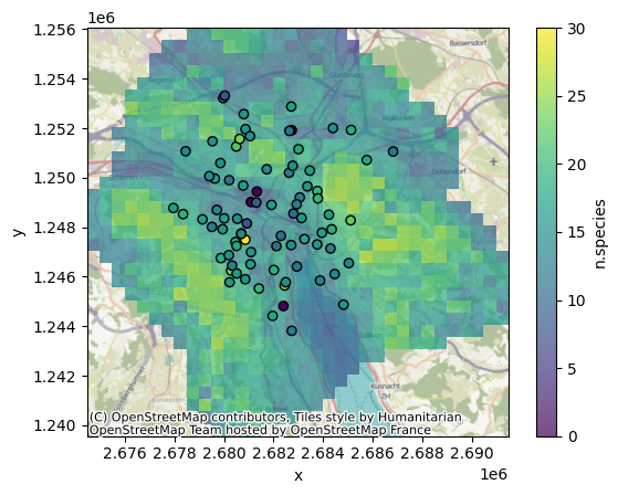
Let us now proceed to the spatial extrapolation of the model based on building volumes and tree canopy:
[ ]:
model_class = linear_model.LinearRegression
urban_model = model_class().fit(urban_fa.features_df, y_ser)
urban_pred_da = urban_fa.predict_raster(
    urban_model,
    study_area_filepath,
    grid_res,
    pred_label=y_ser.name,
)
focalpy.plot_raster_and_gdf(urban_pred_da, bird_gdf, y_ser)
<Axes: xlabel='x', ylabel='y'>
We can actually plot both maps side-by-side with a common color scale:
[ ]:
fig, axes = plt.subplots(1, 2, figsize=(figwidth * 2, figheight))
vmin = min(pred_da.min().item(), urban_pred_da.min().item(), y_ser.min())
vmax = max(pred_da.max().item(), urban_pred_da.max().item(), y_ser.max())
for ax, da, title in zip(
    axes,
    [pred_da, urban_pred_da],
    ["Landscape metrics", "Building and tree predictors"],
):
    focalpy.plot_raster_and_gdf(da, bird_gdf, y_ser, ax=ax, vmin=vmin, vmax=vmax)
    ax.set_title(title)
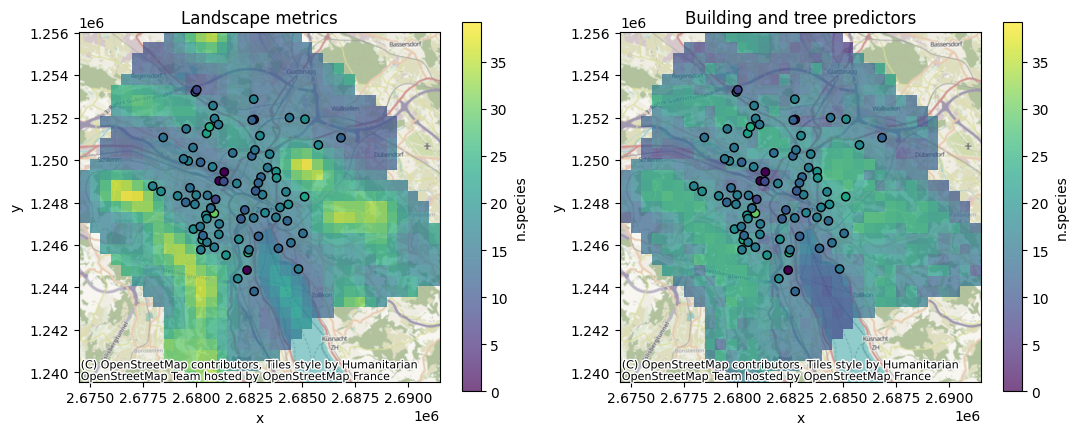
It seems that using the surrounding building volumes and the tree canopy amounts result in a smoother species richness map than its landscape metrics-based counterpart (which is likely in line with the discrete nature of LULC categories).
Finally, note that we can use cross-validation to select any model other than a linear regression:
[ ]:
# compare models using 3-fold cross-validation
model_class_dict = {
    "Linear regression": linear_model.LinearRegression(),
    "Gradient boosting": ensemble.GradientBoostingRegressor(),
    "Random forest": ensemble.RandomForestRegressor(),
}
for name, model in model_class_dict.items():
    scores = cross_val_score(
        model,
        X_urban_df,
        y_ser,
        cv=3,
        scoring=lambda est, X, y: stats.pearsonr(y, est.predict(X))[0] ** 2,
    )
    print(f"{name}: mean R2 = {scores.mean():.3f} (+/- {scores.std():.3f})")
Linear regression: mean R2 = 0.167 (+/- 0.135)
Gradient boosting: mean R2 = 0.094 (+/- 0.107)
Random forest: mean R2 = 0.160 (+/- 0.120)
Nonetheless it seems that the linear regression shows the most robust performance for this relationship.