Land use regression#
The last two decades have seen increasing interest in land use regression (LUR) models (Hoek et al., 2008), which combine spatial predictors related to land use with data collected from monitoring stations, e.g., air pollution or temperature.
In this notebook, we show how the FocalAnalysis class can be used to assess the urban heat island (UHI) effect by predicting air temperature observations from weather stations from MeteoSwiss and the Office of Waste, Water, Energy and Air (AWEL) in Zurich, Switzerland. We will focus on measurements at 9 p.m. - when the UHI effect is estimated to reach its maximum intensity in Swiss urban areas (Burgstall, 2019) - collected during a 5-day heatwave from June 16-20 in 2022
(which corresponds to a level 3 heat warning according to the MeteoSwiss heat warning system, i.e., three or more days with mean temperature over 25 \(^{\circ} C\) (Burgstall et al., 2021).
We will first import the required libraries and define some variables with input file paths and parameters:
[ ]:
import contextily as cx
import geopandas as gpd
import matplotlib.pyplot as plt
import pandas as pd
import statsmodels.api as sm
from sklearn import linear_model, preprocessing

import focalpy
[ ]:
study_area_filepath = "data/study-area.gpkg"
stations_filepath = "data/stations.gpkg"
# netatmo_cws_filepath = "data/netatmo-cws.gpkg"

buildings_filepath = "data/buildings.gpkg"
tree_canopy_filepath = "data/tree-canopy.tif"
dem_filepath = "data/dem.tif"

ts_df_filepath = "data/heatwaves-2022.csv"

y_name = "$\Delta$T$_{mean}$"

grid_res = 500

buffer_dists = [50, 100, 250, 500]
topo_buffer_dists = [250, 500]

# viz
heatmap_kwargs = dict(annot=True, fmt=".2f", cmap="coolwarm", vmin=-1, vmax=1)
figwidth = plt.rcParams["figure.figsize"][0]
figheight = plt.rcParams["figure.figsize"][1]
<>:11: SyntaxWarning: invalid escape sequence '\D'
<>:11: SyntaxWarning: invalid escape sequence '\D'
/tmp/ipykernel_1229499/3644085884.py:11: SyntaxWarning: invalid escape sequence '\D'
  y_name = "$\Delta$T$_{mean}$"
We can start by showing the data frame with the time series of temperature measurements:
[ ]:
ts_df = pd.read_csv(ts_df_filepath, index_col="time", parse_dates=["time"])
ts_df.head()
| 530 | 534 | 2651 | 2652 | 2653 | 2655 | 2656 | 2657 | 2659 | 2679 | ... | 2683 | 2688 | 2689 | 2695 | 2696 | 2697 | 2698 | 2810 | REH | SMA | |
|---|---|---|---|---|---|---|---|---|---|---|---|---|---|---|---|---|---|---|---|---|---|
| time | |||||||||||||||||||||
| 2022-06-16 21:00:00 | 21.866667 | 25.090000 | 22.041667 | 24.926667 | 22.578333 | 23.745000 | 21.856667 | 22.213333 | 24.678333 | 23.503333 | ... | 23.026667 | 22.785000 | 25.118333 | 24.286000 | 22.060000 | 20.572000 | 23.748333 | 21.160000 | 19.566667 | 21.716667 |
| 2022-06-17 21:00:00 | 21.320000 | 23.830000 | 21.565000 | 24.872000 | 19.938333 | 23.716667 | 22.910000 | 22.442500 | 23.753333 | 21.385000 | ... | 22.215000 | 22.915000 | 24.925000 | 24.178333 | 21.976667 | 20.101667 | 24.010000 | 20.845000 | 18.566667 | 21.016667 |
| 2022-06-18 21:00:00 | 23.681667 | 26.655000 | 23.736667 | 27.240000 | 22.731667 | 25.928333 | 26.018333 | 24.455000 | 26.200000 | 23.633333 | ... | 24.400000 | 24.760000 | 27.641667 | 26.760000 | 24.065000 | 22.815000 | 26.643333 | 23.256667 | 20.500000 | 23.400000 |
| 2022-06-19 21:00:00 | 27.363333 | 29.318333 | 27.553333 | 30.608333 | 26.130000 | 30.316667 | 25.961667 | 28.051667 | 29.436667 | 27.260000 | ... | 28.218000 | 29.918333 | 30.813333 | 30.246667 | 29.603333 | 25.312000 | 30.326667 | 26.528333 | 26.533333 | 26.416667 |
| 2022-06-20 21:00:00 | 24.266000 | 24.626667 | 23.390000 | 25.152500 | 21.692500 | 24.483333 | 20.535000 | 24.211667 | 24.531667 | 23.700000 | ... | 23.728333 | 24.143333 | 24.595000 | 24.936667 | 23.956667 | 23.872000 | 24.631667 | 23.793333 | 22.583333 | 22.100000 |
5 rows × 22 columns
as well as the mean (out of all the stations) 9 p.m. temperature of each day:
[ ]:
ts_df.mean(axis="columns").head()
time
2022-06-16 21:00:00    23.072258
2022-06-17 21:00:00    22.514326
2022-06-18 21:00:00    24.929621
2022-06-19 21:00:00    28.454788
2022-06-20 21:00:00    23.884227
dtype: float64
In order to assess the UHI effect, our target variable \(y := \Delta\)T\(_{mean}\) for each station will be the difference between its temperature and the mean of the concurrent temperatures:
[ ]:
y_ser = ts_df.sub(ts_df.mean(axis="columns"), axis="index").mean().rename(y_name)
y_ser.head()
530    -0.681919
534     1.287057
2651   -0.913134
2652    1.808307
2653   -2.162574
Name: $\Delta$T$_{mean}$, dtype: float64
Let us now load the station locations and plot them by data source:
[ ]:
stations_gdf = gpd.read_file(stations_filepath).set_index("station_id")
# select only stations with valid temperature data
stations_gdf = stations_gdf.loc[y_ser.index]
# stations_gdf.head()
ax = stations_gdf.plot(column="source", legend=True)
cx.add_basemap(ax, crs=stations_gdf.crs)

We can also plot them by their difference with the mean 9 p.m. temperature \(\Delta\)T\(_{mean}\):
[ ]:
# station_gdf.plot(ts_df.mean(), legend=True, cmap="coolwarm")
ax = stations_gdf.assign(**{y_name: y_ser}).plot(
    y_name,
    legend=True,
    cmap="coolwarm",
    edgecolor="k",
    legend_kwds={"label": f"{y_name} $\:$ [$\circ$C]"},
)
cx.add_basemap(ax, crs=stations_gdf.crs)
<>:7: SyntaxWarning: invalid escape sequence '\:'
<>:7: SyntaxWarning: invalid escape sequence '\:'
/tmp/ipykernel_1229499/1897662534.py:7: SyntaxWarning: invalid escape sequence '\:'
  legend_kwds={"label": f"{y_name} $\:$ [$\circ$C]"},

Spatial predictors#
In line with related works, e.g., (Burger et al., 2021), for each station location we will compute a set of spatial predictors, i.e., building volume, tree canopy and two of topographic features, namely the slope and topographic position index (TPI).
Like in the focal site multi-scale study framework for landscape-species inference (Brennen et al., 2002), spatial predictors in LURs are also often computed for concentric circular buffers around each station. For the building volume and tree canopy, the radii (scale) are 50, 100, 250 and 500 m, whereas for the topographic features the smallest scales of 50 and 100 m are excluded since it is consider unlikely to reflect the upwind fetch required for air at screen height to adjust to its underlying surface (Stewart and Oke, 2012).
[ ]:
building_gdf = gpd.read_file(buildings_filepath).set_index("id")
# add a "volume" column
building_gdf["volume"] = building_gdf["area"] * building_gdf["height"]
# building_gdf.head()

fa = focalpy.FocalAnalysis(
    [building_gdf, tree_canopy_filepath, dem_filepath],
    stations_gdf,
    [buffer_dists, buffer_dists, topo_buffer_dists],
    [
        "compute_vector_features",
        "compute_raster_features",
        "compute_terrain_attributes",
    ],
    feature_col_prefixes=["building", "tree", ""],
    feature_methods_args={
        "compute_vector_features": [{"volume": "sum"}],
        "compute_terrain_attributes": [["slope", "topographic_position_index"]],
    },
    feature_methods_kwargs={
        "compute_raster_features": {"stats": "sum"},
        "compute_terrain_attributes": {"stats": "mean"},
    },
)
fa.features_df.head()
| building_volume_sum_50 | building_volume_sum_100 | building_volume_sum_250 | building_volume_sum_500 | tree_sum_50 | tree_sum_100 | tree_sum_250 | tree_sum_500 | slope_mean_250 | slope_mean_500 | topographic_position_index_mean_250 | topographic_position_index_mean_500 | |
|---|---|---|---|---|---|---|---|---|---|---|---|---|
| 530 | 3248.321176 | 39068.509901 | 2.568809e+05 | 1.397370e+06 | 1203.0 | 3924.0 | 22994.0 | 84803.0 | 6.819450 | 6.884670 | -0.000910 | -0.000199 |
| 534 | 37349.677706 | 262285.820827 | 2.058157e+06 | 5.205767e+06 | 303.0 | 1294.0 | 5673.0 | 26121.0 | 2.195517 | 3.457119 | 0.000024 | 0.000003 |
| 2651 | 42799.252900 | 130087.412717 | 5.394371e+05 | 1.874661e+06 | 650.0 | 2281.0 | 12913.0 | 59364.0 | 3.865617 | 3.948312 | 0.000070 | -0.000084 |
| 2652 | 28891.012664 | 100381.131949 | 6.930643e+05 | 2.925047e+06 | 134.0 | 1607.0 | 10679.0 | 38572.0 | 3.354241 | 3.435203 | -0.000046 | -0.000022 |
| 2653 | 8218.052929 | 39102.191933 | 3.850106e+05 | 1.081819e+06 | 845.0 | 3211.0 | 18900.0 | 83168.0 | 6.210232 | 8.461916 | 0.000689 | 0.000174 |
We can fit a linear regression using ordinary least squares (OLS) with statsmodels to get a first grasp of the relationship:
[ ]:
# first, standardize features. Note that we need to keep the data frame index/columns
X_df = pd.DataFrame(
    preprocessing.StandardScaler().fit_transform(fa.features_df),
    index=fa.features_df.index,
    columns=fa.features_df.columns,
)

# linear regression with statsmodels OLS
results = sm.OLS(y_ser, sm.add_constant(X_df)).fit()
print(results.summary())
                            OLS Regression Results
==============================================================================
Dep. Variable:     $\Delta$T$_{mean}$   R-squared:                       0.900
Model:                            OLS   Adj. R-squared:                  0.767
Method:                 Least Squares   F-statistic:                     6.769
Date:                Wed, 31 Dec 2025   Prob (F-statistic):            0.00370
Time:                        15:38:28   Log-Likelihood:                -14.815
No. Observations:                  22   AIC:                             55.63
Df Residuals:                       9   BIC:                             69.81
Df Model:                          12
Covariance Type:            nonrobust
=======================================================================================================
                                          coef    std err          t      P>|t|      [0.025      0.975]
-------------------------------------------------------------------------------------------------------
const                                4.718e-16      0.158   2.98e-15      1.000      -0.358       0.358
building_volume_sum_50                  0.1496      0.351      0.426      0.680      -0.644       0.943
building_volume_sum_100                 0.5653      0.618      0.915      0.384      -0.833       1.964
building_volume_sum_250                 0.1683      0.755      0.223      0.828      -1.539       1.875
building_volume_sum_500                 0.5257      0.717      0.733      0.482      -1.097       2.148
tree_sum_50                            -0.5796      0.650     -0.892      0.396      -2.050       0.891
tree_sum_100                            0.1980      1.344      0.147      0.886      -2.843       3.239
tree_sum_250                            0.5707      1.828      0.312      0.762      -3.564       4.705
tree_sum_500                           -0.4014      1.166     -0.344      0.739      -3.040       2.237
slope_mean_250                          4.0204      1.824      2.204      0.055      -0.106       8.147
slope_mean_500                         -3.7181      2.115     -1.758      0.113      -8.502       1.066
topographic_position_index_mean_250    -0.5917      0.359     -1.650      0.133      -1.403       0.220
topographic_position_index_mean_500     0.7722      0.296      2.605      0.029       0.102       1.443
==============================================================================
Omnibus:                        1.178   Durbin-Watson:                   2.284
Prob(Omnibus):                  0.555   Jarque-Bera (JB):                1.052
Skew:                           0.368   Prob(JB):                        0.591
Kurtosis:                       2.222   Cond. No.                         57.3
==============================================================================

Notes:
[1] Standard Errors assume that the covariance matrix of the errors is correctly specified.
While we have a very strong fit as indicated by the coefficient of determination R\(^2 = 0.9\), the condition number is very high, suggesting strong collinearity of spatial predictors, which is very common in environmental data and in this example is further exacerbated by including the same predictors computed at multiple scales.
Scale of influence#
In a very similar way to landscape-species studies, a common practice in LURs is to select the scale (e.g., buffer radii) at which each spatial predictor shows the strongest relationship the response variable. In landscape-species relationships, this is called the “scale of effect” (Jackson and Fahrig, 2012), whereas LURs often use the “scale of influence” term (Llaguno-Munitxa and Bou-Zeid, 2020). We can use the scale_eval_ser function to evaluate the strength of the relationship at each scale:
[ ]:
focalpy.scale_eval_ser(X_df, y_ser, how="individual")
building_volume_sum              building_volume_sum_50                 0.284406
                                 building_volume_sum_100                0.315045
                                 building_volume_sum_250                0.503243
                                 building_volume_sum_500                0.571616
slope_mean                       slope_mean_250                         0.023251
                                 slope_mean_500                         0.038490
topographic_position_index_mean  topographic_position_index_mean_250    0.101497
                                 topographic_position_index_mean_500    0.013587
tree_sum                         tree_sum_50                            0.163510
                                 tree_sum_100                           0.229503
                                 tree_sum_250                           0.218702
                                 tree_sum_500                           0.181388
Name: rsquared, dtype: float64
which suggests that the strongest effects occur at the 500 m scale for buildings, 100 m for trees, 500 m for the slope and 250 m for the TPI. We can get the list of features at their scale of influence (based on the evaluation shown above) using the scale_of_effect_features, which will return the column names:
[ ]:
soe_features = focalpy.scale_of_effect_features(fa.features_df, y_ser, how="individual")
soe_features
array(['building_volume_sum_500', 'slope_mean_500',
       'topographic_position_index_mean_250', 'tree_sum_100'],
      dtype=object)
which we can now use to perform again our regression using only the features at their scale of influence:
[ ]:
results = sm.OLS(y_ser, sm.add_constant(X_df[soe_features])).fit()
print(results.summary())
                            OLS Regression Results
==============================================================================
Dep. Variable:     $\Delta$T$_{mean}$   R-squared:                       0.684
Model:                            OLS   Adj. R-squared:                  0.610
Method:                 Least Squares   F-statistic:                     9.214
Date:                Wed, 31 Dec 2025   Prob (F-statistic):           0.000377
Time:                        15:39:46   Log-Likelihood:                -27.487
No. Observations:                  22   AIC:                             64.97
Df Residuals:                      17   BIC:                             70.43
Df Model:                           4
Covariance Type:            nonrobust
=======================================================================================================
                                          coef    std err          t      P>|t|      [0.025      0.975]
-------------------------------------------------------------------------------------------------------
const                                4.718e-16      0.205    2.3e-15      1.000      -0.432       0.432
building_volume_sum_500                 1.0109      0.247      4.086      0.001       0.489       1.533
slope_mean_500                          0.9639      0.403      2.394      0.028       0.115       1.813
topographic_position_index_mean_250    -0.5682      0.329     -1.726      0.102      -1.263       0.126
tree_sum_100                           -0.5676      0.322     -1.760      0.096      -1.248       0.113
==============================================================================
Omnibus:                        0.528   Durbin-Watson:                   2.340
Prob(Omnibus):                  0.768   Jarque-Bera (JB):                0.068
Skew:                           0.132   Prob(JB):                        0.967
Kurtosis:                       3.063   Cond. No.                         4.11
==============================================================================

Notes:
[1] Standard Errors assume that the covariance matrix of the errors is correctly specified.
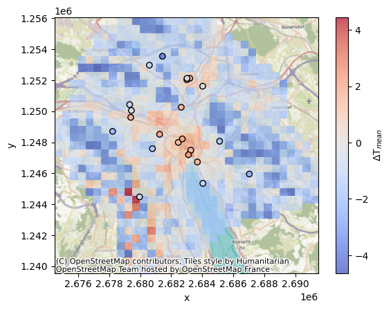
As we can see, although selecting the features at their scale of influence results in a lower yet still moderate R\(^2\), the condition number is notably reduced, no longer indicating an issue of multicollinearity. Additionally, we can see that the building volume and slope have a positive effect on \(\Delta\)T\(_{mean}\), i.e., are associated with higher temperatures whereas the opposite holds for the tree canopy and TPI.
Finally, we can use the fitted linear regression model to spatially extrapolate the LUR to our entire study area using the predict_raster function:
[ ]:
model = linear_model.LinearRegression().fit(fa.features_df[soe_features], y_ser)
pred_da = fa.predict_raster(
    model, study_area_filepath, grid_res, features=soe_features, pred_label=y_name
)
# plot the raster
focalpy.plot_raster_and_gdf(pred_da, stations_gdf, y_ser, cmap="coolwarm")
<Axes: xlabel='x', ylabel='y'>